3D-MNIST Image Classification

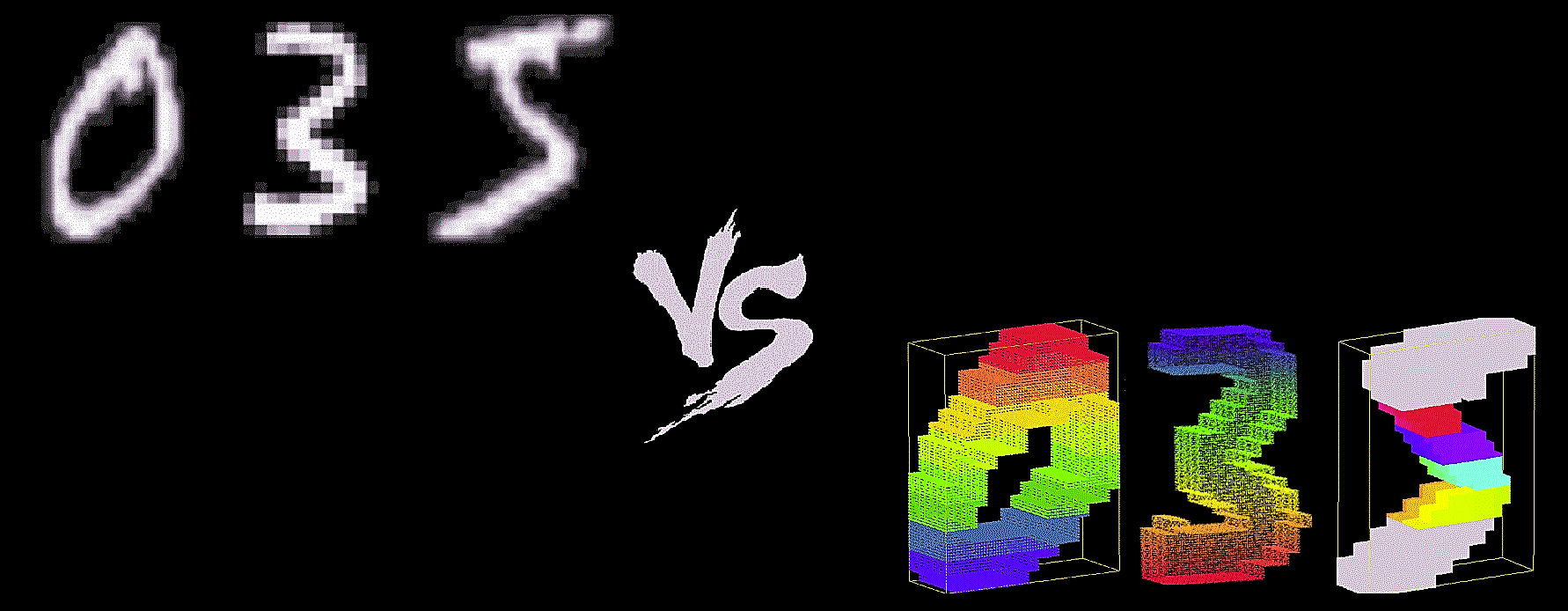
By Shashwat Aggarwal on January 12, 2018.

Introduction

The MNIST [1] is the de facto “hello world” dataset for anyone getting started with computer vision. It contains a total of 70,000 examples divided into training and testing sets (6:1). Since its release in 1999, this classic dataset of handwritten images has served as the basis for benchmarking classification algorithms. Various emerging machine learning techniques have been tested with the MNIST, that has remained a reliable resource for researchers and learners alike. More recently, Convolutional Neural Networks (CNN), a class of Deep Neural Networks have demonstrated immense success in the field of computer vision [2]. The MNIST dataset, in particular, has been effectively classified using architectures of this type, with the current state-of-the-art at a high 99.79% accuracy [3].

MNIST is a good database for people who want to get acquainted with computer vision and pattern recognition methods to solve real-world problems, but most of the real-world vision problems like autonomous robots and scene understanding deal with 3D datasets. The availability of 3D data has been increasing rapidly as the use of sensors which provide 3D spatial readings in autonomous vehicles and robots becomes more prevalent. For this reason, the ability of these machines to automatically identify and make inferences about this data has become a crucial task for them to operate autonomously.

Recently, a 3D version of the MNIST was released on Kaggle [4]. The dataset was created by generating 3D point clouds from the images of the digits in the original 2D MNIST. The script for generating point clouds can be found here. This dataset can be considered as a good starting point for getting familiar with 3D vision tasks. In this blog post, we explore this dataset and empirically compare the performance of various machine learning and deep learning based algorithms for the classification of 3D digits.

Overview of 3D MNIST Dataset

The 3D MNIST dataset is available in HDF5 file format, here. The dataset contains 3D point clouds, i.e., sets of (x, y, z) coordinates generated from a portion of the original 2D MNIST dataset (around 5,000 images). The point clouds have zero mean and a maximum dimension range of 1. Each HDF5 group contains:

• “points” dataset: x, y, z coordinates of each 3D point in the point cloud.
• “normals” dataset: nx, ny, nz components of the unit normal associate to each point.
• “img” dataset: the original MNIST image.
• “label” attribute: the original MNIST label.

In addition to train and test point clouds, the dataset also contains full_dataset_vectors.h5 that stores 4096-D vectors obtained from voxelization of all the 3D point clouds and their randomly rotated copies with noise. The full_dataset_vectors.h5 is splitted into 4 groups:

X_train = f["X_train"][:]    # shape: (10000, 4096)
y_train = f["y_train"][:]    # shape: (10000,)   
X_test  = f["X_test"][:]     # shape: (2000, 4096) 
y_test  = f["y_test"][:]     # shape: (2000,)

Here is an example to read a digit and store its group content in a tuple.

with h5.File('train_point_clouds.h5', 'r') as f:  
    # Reading digit at zeroth index      
    a = f["0"]     
    # Storing group contents of digit a  
    digit = (a["img"][:], a["points"][:], a.attrs["label"])

Let’s first visualize the contents stored in the tuple with matplotlib. The following code plots the first 15 images from the original 2D MNIST with their corresponding labels:

# Plot some examples from original 2D-MNIST  
fig, ax = plt.subplots(3,5, figsize=(12, 12), facecolor='w', edgecolor='k')

fig.subplots_adjust(hspace = .5, wspace=.2)

for ax, d in zip(axs.ravel(), digits):  
    ax.imshow(d[0][:])  
    ax.set_title("Digit: " + str(d[2]))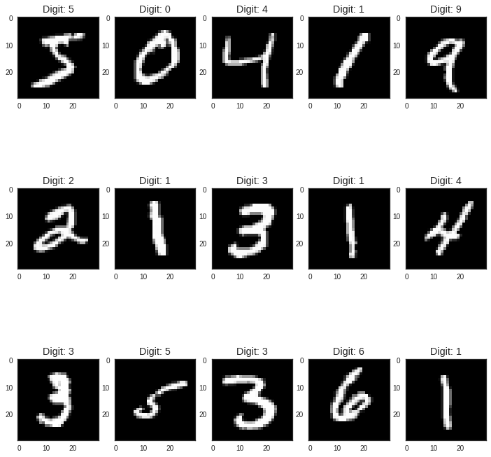

Before visualizing the 3D point clouds, let’s first discuss about Voxelization. Voxelization is the process of conversion of a geometric object from its continuous geometric representation into a set of voxels that best approximates the continuous object. The process mimics the scan-conversion process that rasterizes 2D geometric objects, and is also referred to as 3D scan-conversion.

We use this process to fit an axis-aligned bounding box called the Voxel Grid around the point clouds and subdivide the grid into segments, assigning each point in the point cloud to one of the sub boxes (known as voxels, analogous to pixels). We split the grid into 16 segments along each axis resulting in a total of 4096 voxels, equivalent to the 4th level of an Octree.

voxel_grid = VoxelGrid(digit, x_y_z = [16, 16, 16])

The code above generates a voxel grid of 16 × 16 × 16 = 4096 voxels, with the structure attribute representing a 2D array, where each row represents a point in the original point cloud and each column represents the n_voxel where it lies with respect to [x_axis, y_axis, z_axis, global].

voxel_grid.structure[0]

array([ 5, 3, 7, 477])

The histogram shown below visualize the number of points present within each voxel. From the plot, it can be seen that there are a lot of empty voxels. This is due to the use of a cuboid bounding box to ensure that the Voxel Grid will divide the cloud in a similar way even when the point clouds are oriented to different directions.

# Get the count of points within each voxel.  
plt.title("DIGIT: " + str(digits[0][-1]))  
plt.xlabel("VOXEL")  
plt.ylabel("POINTS INSIDE THE VOXEL")  
count_plot(voxels[0].structure[:,-1])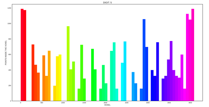   

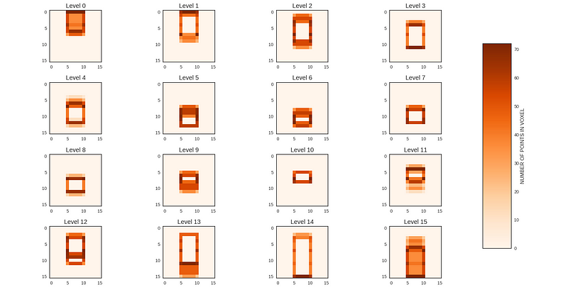
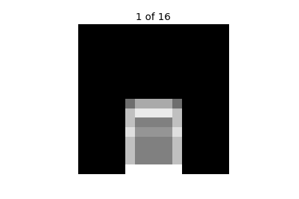
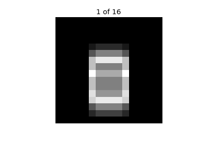
We can visualize the Voxel Grid using the built-in helper function plot() defined in the file plot3D.py provided along with the dataset. This function displays the sliced spatial views of the Voxel Grid around the z-axis.

>>> # Visualizing the Voxel Grid sliced around the z-axis.

>>> voxels[0].plot()  
>>> plt.show()

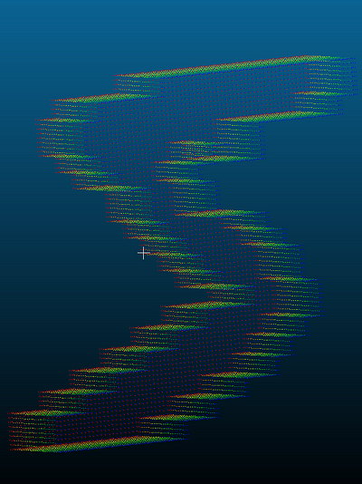
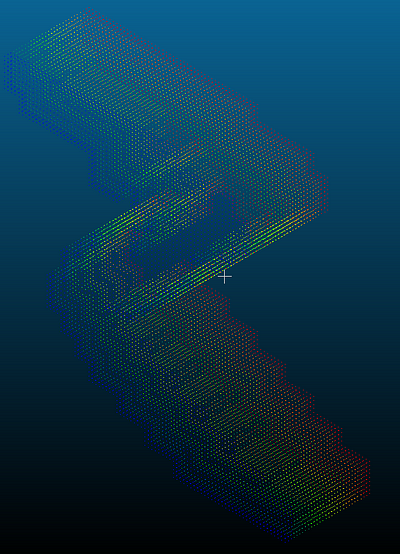
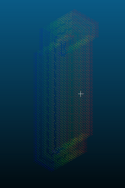
Now we visualize the 3D point clouds using an open-source 3D software, CloudCompare. We save the Voxel Grid structure as the scalar fields of the original point clouds and render 3D images with CloudCompare.

>>> # Save Voxel Grid Structure as the scalar field of Point Cloud.  
>>> cloud_vis = np.concatenate((digit[1], voxel_grid.structure), axis=1)

>>> np.savetxt('Cloud Visualization - ' + str(digit[2]) + '.txt', cloud_vis)

At last, before moving on to the classification task, just for fun, let’s visualize the animation of 3D data slice by slice. Both the rows of the plot show the animation of slices along x, y, z-axis for the digits 5 and 0.

Sklearn Machine Learning Classifiers

We use the full_vectors.h5 dataset. You can use this or generate your own using this script. In machine learning, there’s something called the “No Free Lunch” theorem that in a nutshell, states that no one algorithm works best for every problem. So we try many machine learning algorithms and choose the best suited to our problem.

Let’s start with the simplest yet powerful machine learning classifier — Logistic Regression:

>>> reg = LogisticRegression()  
>>> reg.fit(X_train, y_train)  
>>> print("Accuracy: ", reg.score(X_test, y_test))

Accuracy: 0.582

Logistic Regression provides a decent baseline for other classifiers with an test-accuracy score of 58.2%.

Next we move on to Decision Trees:

>>> dt = DecisionTreeClassifier()  
>>> dt.fit(X_train, y_train)  
>>> print("Accuracy: ", dt.score(X_test, y_test))

Accuracy: 0.4865

Decision Trees gives a test-accuracy of 48.65%, i.e. 10 points lower as compared to Logistic Regression. The performance of Decision Trees can possibly be improved with hyper-parameter tuning and grid-search. But here, we stick to the basics and try to get a rough estimate of the performance of the classifier.

Moving further, let’s try Support Vector Machines:

>>> svm = LinearSVC()  
>>> svm.fit(X_train, y_train)  
>>> print("Accuracy: ", svm.score(X_test, y_test))

Accuracy: 0.557

We use linear SVMs instead of RBF or Poly kernel based SVM as they take a lot of time to train (you may try training these SVM variants and compare their performance against other classifiers). Linear SVMs perform similar to Logistic Regression with a test-accuracy score of 55.7%.

Now, giving K Nearest Neighbors a shot!

>>> knn = KNN()  
>>> knn.fit(X_train, y_train)  
>>> print("Accuracy: ", knn.score(X_test, y_test))

Accuracy: 0.5905

KNN performs best among all the previously tried classifiers with 59.05% test-score.

Finally, let’s ensemble; Random Forests:

>>> rf = RandomForestClassifier(n_estimators=500)  
>>> rf.fit(X_train, y_train)  
>>> print("Accuracy: ", rf.score(X_test, y_test))

Accuracy: 0.685

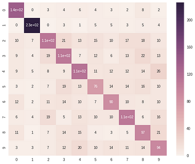
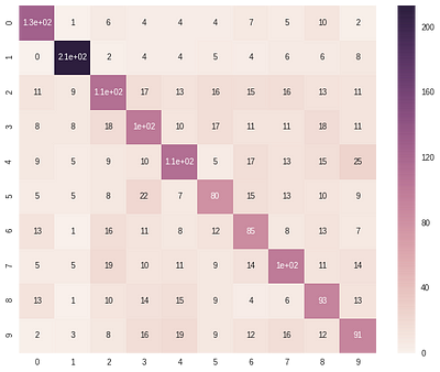
Random Forests outperforms all other classifiers on the classification task. The table below reports the test-accuracy of each classifier on the 3D MNIST dataset. The confusion matrix plots shown below, provides us with the classification report summary of three classifiers namely, Logistic Regression, SVM and Random Forests. From these plots, we observe that most of the classifiers experience difficulty in classifying digits 5, 6 and 9 correctly while find classifying digits like 0, 1 and 4 easy.

You can find the complete code for ML-based empirical analysis here. Although Random Forests performs best among the tried classifiers, the 68.5% mark seems way behind its score on the 2D equivalent dataset. So the natural question that arrives is can we do better?

Moving on to Convolutional Neural Networks

Convolutional Neural Networks (CNN), have been immensely successful in classifying the 2D version of MNIST, with the current state-of-the-art model giving a high 99.79% accuracy. So now, let’s see how well these CNN perform with the 3D equivalent of MNIST. We create a 4-layered CNN in keras with two dense layers at the top. For the complete definition of the model, look at the model() method. Since a sample in our dataset is a 4096-D voxel and CNN expects a 4D tensor of shape: (batch_size, height, width, input_channels), so we reshape our dataset into a 4D tensor: (-1, 16, 16, 16).

We tried several other shapes such as (-1, 64, 64, 1), (-1, 64, 64, 3) but (-1, 16, 16, 16) gave the best results, so we stick with this.

{ % gist imshashwataggarwal/9a4eabf0d03ef755060a5d4b82ef3875#file-2dcnn-py % }

Output

Epoch 1/30  
3s - loss: 2.0299 - acc: 0.2922 - val\_loss: 2.2644 - val\_acc: 0.1960  
Epoch 2/30  
3s - loss: 1.4517 - acc: 0.4913 - val\_loss: 2.0336 - val\_acc: 0.4440  
Epoch 3/30  
3s - loss: 1.3081 - acc: 0.5364 - val\_loss: 1.6669 - val\_acc: 0.5140  
Epoch 4/30  
3s - loss: 1.2385 - acc: 0.5595 - val\_loss: 1.4951 - val\_acc: 0.5667  
Epoch 5/30  
3s - loss: 1.1959 - acc: 0.5799 - val\_loss: 1.2812 - val\_acc: 0.5813  
Epoch 6/30  
3s - loss: 1.1682 - acc: 0.5826 - val\_loss: 1.1254 - val\_acc: 0.6053  
Epoch 7/30  
3s - loss: 1.1552 - acc: 0.5909 - val\_loss: 1.0595 - val\_acc: 0.6240  
Epoch 8/30  
3s - loss: 1.1247 - acc: 0.6008 - val\_loss: 0.9993 - val\_acc: 0.6460  
Epoch 9/30  
3s - loss: 1.0981 - acc: 0.6142 - val\_loss: 0.9978 - val\_acc: 0.6313  
Epoch 10/30  
3s - loss: 1.0928 - acc: 0.6103 - val\_loss: 0.9892 - val\_acc: 0.6527  
Epoch 11/30  
3s - loss: 1.0770 - acc: 0.6202 - val\_loss: 0.9940 - val\_acc: 0.6387  
Epoch 12/30  
3s - loss: 1.0627 - acc: 0.6215 - val\_loss: 0.9916 - val\_acc: 0.6573  
Epoch 13/30  
3s - loss: 1.0704 - acc: 0.6239 - val\_loss: 1.0423 - val\_acc: 0.6400  
Epoch 14/30  
3s - loss: 1.0524 - acc: 0.6296 - val\_loss: 0.9560 - val\_acc: 0.6573  
Epoch 15/30  
3s - loss: 1.0331 - acc: 0.6320 - val\_loss: 0.9504 - val\_acc: 0.6540  
Epoch 16/30  
3s - loss: 1.0215 - acc: 0.6353 - val\_loss: 0.9428 - val\_acc: 0.6800  
Epoch 17/30  
3s - loss: 1.0052 - acc: 0.6461 - val\_loss: 0.9492 - val\_acc: 0.6633  
Epoch 18/30  
3s - loss: 1.0090 - acc: 0.6389 - val\_loss: 0.9468 - val\_acc: 0.6693  
Epoch 19/30  
3s - loss: 0.9957 - acc: 0.6520 - val\_loss: 0.9322 - val\_acc: 0.6700  
Epoch 20/30

Epoch 00019: reducing learning rate to 0.000500000023749.

3s - loss: 0.9831 - acc: 0.6507 - val\_loss: 0.9482 - val\_acc: 0.6653  
Epoch 21/30  
3s - loss: 0.9643 - acc: 0.6636 - val\_loss: 0.8976 - val\_acc: 0.6767  
Epoch 22/30  
3s - loss: 0.9341 - acc: 0.6679 - val\_loss: 0.8920 - val\_acc: 0.6873  
Epoch 23/30  
3s - loss: 0.9078 - acc: 0.6785 - val\_loss: 0.8755 - val\_acc: 0.6933  
Epoch 24/30  
3s - loss: 0.9386 - acc: 0.6650 - val\_loss: 0.8968 - val\_acc: 0.6840  
Epoch 25/30  
3s - loss: 0.9130 - acc: 0.6792 - val\_loss: 0.8872 - val\_acc: 0.6900  
Epoch 26/30  
3s - loss: 0.8946 - acc: 0.6765 - val\_loss: 0.8736 - val\_acc: 0.6960  
Epoch 27/30  
3s - loss: 0.8997 - acc: 0.6785 - val\_loss: 0.8668 - val\_acc: 0.7060  
Epoch 28/30  
3s - loss: 0.8802 - acc: 0.6879 - val\_loss: 0.8859 - val\_acc: 0.6853  
Epoch 29/30  
3s - loss: 0.8877 - acc: 0.6890 - val\_loss: 0.8732 - val\_acc: 0.6967  
Epoch 30/30  
3s - loss: 0.8832 - acc: 0.6858 - val\_loss: 0.8768 - val\_acc: 0.6913

Accuracy : 0.698

3D Convolutional Networks in Keras

Finally, we move onto the main objective of this post (:P), 3D CNN. The 3D CNN model is similar to our 2D CNN model. For the complete definition of the model, check the model() method. Now, like with 2D CNN, the 3D CNN expects a 5D tensor of shape (batch_size, conv_dim1, conv_dim2, conv_dim3, input_channels). We reshape out input to a 5D tensor — (-1, 16, 16, 16, 3)and feed it to our 3D CNN.

{ % gist imshashwataggarwal/89e78280267bfd6bf195707ff9b47d93#file-3d_cnn-py % }

Output

Epoch 1/30  
11s- loss: 2.1194 - acc: 0.2912 - val\_loss: 2.1434 - val\_acc: 0.1660  
Epoch 2/30  
10s- loss: 1.3554 - acc: 0.5274 - val\_loss: 1.8831 - val\_acc: 0.4933  
Epoch 3/30  
10s- loss: 1.1520 - acc: 0.5954 - val\_loss: 2.0278 - val\_acc: 0.3427  
Epoch 4/30  
10s- loss: 1.0604 - acc: 0.6272 - val\_loss: 1.3859 - val\_acc: 0.5500  
Epoch 5/30  
10s- loss: 0.9991 - acc: 0.6448 - val\_loss: 1.2405 - val\_acc: 0.6000  
Epoch 6/30  
10s- loss: 0.9305 - acc: 0.6756 - val\_loss: 1.0759 - val\_acc: 0.6113  
Epoch 7/30  
10s- loss: 0.8790 - acc: 0.6939 - val\_loss: 1.0644 - val\_acc: 0.6673  
Epoch 8/30  
10s- loss: 0.8295 - acc: 0.7087 - val\_loss: 0.8908 - val\_acc: 0.6920  
Epoch 9/30  
10s- loss: 0.7648 - acc: 0.7289 - val\_loss: 0.9673 - val\_acc: 0.6940  
Epoch 10/30  
10s- loss: 0.7001 - acc: 0.7542 - val\_loss: 0.8410 - val\_acc: 0.7047  
Epoch 11/30  
10s- loss: 0.6485 - acc: 0.7719 - val\_loss: 0.8781 - val\_acc: 0.7133  
Epoch 12/30  
10s- loss: 0.5999 - acc: 0.7912 - val\_loss: 0.8172 - val\_acc: 0.7180  
Epoch 13/30  
10s- loss: 0.5375 - acc: 0.8147 - val\_loss: 0.8366 - val\_acc: 0.7207  
Epoch 14/30  
10s- loss: 0.4936 - acc: 0.8284 - val\_loss: 0.8288 - val\_acc: 0.7193  
Epoch 15/30  
10s- loss: 0.4337 - acc: 0.8494 - val\_loss: 0.8528 - val\_acc: 0.7320  
Epoch 16/30  
10s- loss: 0.4099 - acc: 0.8593 - val\_loss: 1.0491 - val\_acc: 0.6907  
Epoch 17/30  
10s- loss: 0.3601 - acc: 0.8764 - val\_loss: 0.9005 - val\_acc: 0.7333  
Epoch 18/30  
10s- loss: 0.3492 - acc: 0.8838 - val\_loss: 0.9155 - val\_acc: 0.7060  
Epoch 19/30  
10s- loss: 0.2939 - acc: 0.9000 - val\_loss: 1.2862 - val\_acc: 0.7007  
Epoch 20/30  
10s- loss: 0.2837 - acc: 0.9058 - val\_loss: 0.9119 - val\_acc: 0.7093  
Epoch 21/30

Epoch 00020: reducing learning rate to 0.000500000023749.

10s- loss: 0.2786 - acc: 0.9104 - val\_loss: 0.9305 - val\_acc: 0.7287  
Epoch 22/30  
10s- loss: 0.1521 - acc: 0.9508 - val\_loss: 1.0142 - val\_acc: 0.7473  
Epoch 23/30  
10s- loss: 0.0944 - acc: 0.9699 - val\_loss: 1.0704 - val\_acc: 0.7300  
Epoch 24/30  
10s- loss: 0.0831 - acc: 0.9746 - val\_loss: 1.1331 - val\_acc: 0.7407  
Epoch 25/30  
10s- loss: 0.0691 - acc: 0.9773 - val\_loss: 1.1615 - val\_acc: 0.7393  
Epoch 26/30

Epoch 00025: reducing learning rate to 0.000250000011874.

10s- loss: 0.0665 - acc: 0.9785 - val\_loss: 1.1331 - val\_acc: 0.7340  
Epoch 27/30  
10s- loss: 0.0468 - acc: 0.9856 - val\_loss: 1.1230 - val\_acc: 0.7367  
Epoch 28/30  
10s- loss: 0.0347 - acc: 0.9888 - val\_loss: 1.1312 - val\_acc: 0.7460  
Epoch 29/30

Epoch 00028: reducing learning rate to 0.000125000005937.

10s- loss: 0.0283 - acc: 0.9919 - val\_loss: 1.1361 - val\_acc: 0.7340  
Epoch 30/30  
10s- loss: 0.0285 - acc: 0.9906 - val\_loss: 1.1466 - val\_acc: 0.7327

Accuracy: 0.771

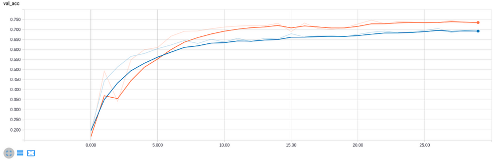
The performance of 2D CNN is close to Random Forests with a test-score of 69.8%, but 3D CNN outperforms all other classifiers by a significant margin, giving a high 77.1% test-accuracy. Below we summarise the classification reports of 2D CNN and 3D CNN through their confusion matrix plots and learning curves respectively.

More 3D Datasets

In this blog post, we experimented with 3D MNIST dataset, that proved to be a good benchmark for starting with 3D Datasets. Here is a list of few more 3D Datasets that are worth playing with:

1. Data Science Bowl 2017, available here.
2. The Joint 2D-3D-Semantic (2D-3D-S) Dataset, available here.
3. The Street View Image, Pose, and 3D Cities Dataset, available here, Project page.
4. The Stanford Online Products dataset, available here.
5. The ObjectNet3D Dataset, available here.
6. The Stanford Drone Dataset, available here.
7. More Datasets.

References

1. The MNIST database of handwritten digits. Y LeCun, C Cortes. 1998.
2. ImageNet classification with deep convolutional neural networks. A. Krizhevsky and I. Sutskever and G. Hinton. NIPS, 2012.
3. Regularization of neural networks using dropconnect. L. Wan and M. Zeiler and S. Zhang and Y. L. Cun and R. Fergus. ICML, 2013.
4. 3D MNIST Dataset. https://www.kaggle.com/daavoo/3d-mnist/data.
5. Voxel. https://en.wikipedia.org/wiki/Voxel#/media/File:Voxels.svg.
6. 3D convolutional neural networks for human action recognition. S. Ji and W. Xu and M. Yang and K. Yu. ICML, 2010.
7. HDF5 File Format. https://support.hdfgroup.org/HDF5/whatishdf5.html
8. Scikit-learn: Machine Learning in Python. Pedregosa et al. JMLR 12, 2011.
9. Keras, https://github.com/fchollet/keras. François Chollet. GitHub, 2015.
10. Stanford Computational Vision and Geometry Lab, http://cvgl.stanford.edu/resources.html

Shashwat Aggarwal

Software Engineering Intern @Microsoft | Computer Science Undergradaute

Tweet Share